Gallery
Some examples of displays, using the R libraries highcharter, reactable, reactablefmtr, to visualize the results of the calculations.
Detailed codes available in the Get Started section.
1) Projected Inventories
a) Simple Table
The light_proj_inv() function allows to calculate quickly the projected inventories and coverages :
for a SKU or a group of SKUs
at an aggregated level (a Product Family or a Storage Location for example)
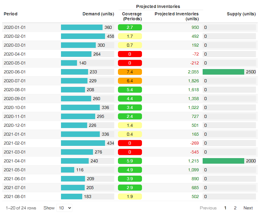
Here is an example of display of table :
we have the 5 initial variables : DFU / Period / Demand (Forecasts) / Opening Inventories / (projected) Supply Plan
and the 2 new features for the DFU : projected inventories & coverages, calculated based on the Demand Forecasts
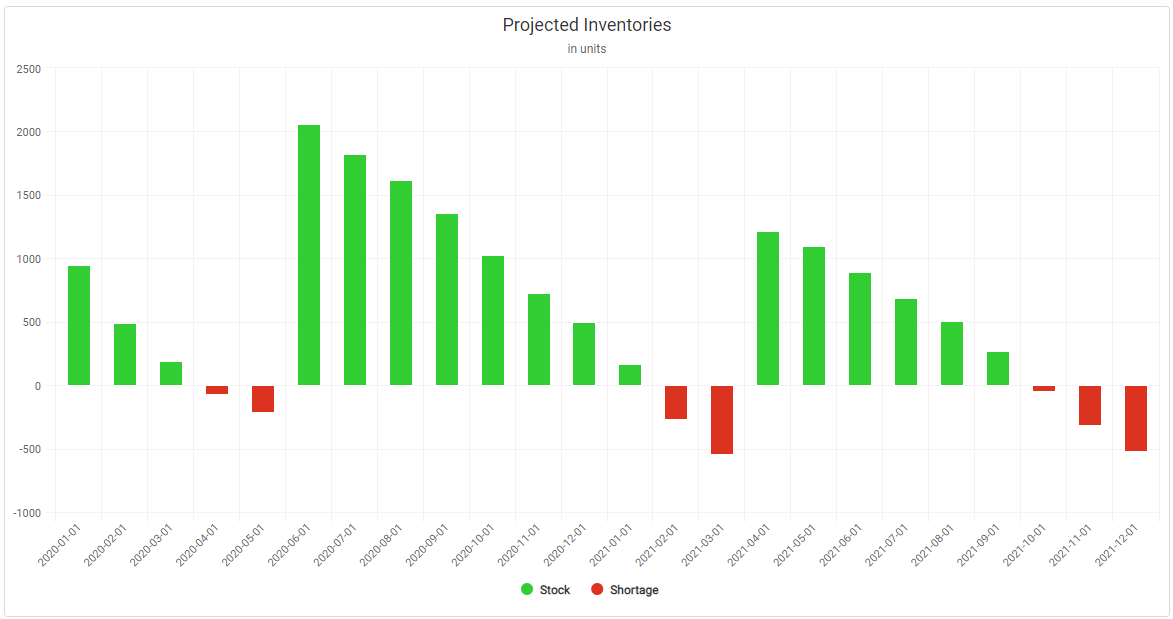
b) Chart
It’s possible to look at the projected inventories in a more visual way, highlighting the periods with shortages :
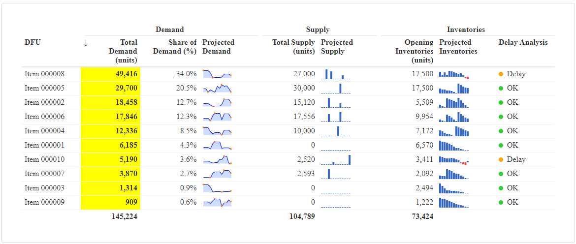
c) Cockpit
If we perform a calculation for several products, we can use a cockpit to get an overview.
Here an example, where the 2 columns on the right give us :
a glimpse of the Projected Inventories for each product (DFU)
an info whether over this horizon we can expect some Delays (i.e. negative inventories) or if everything is fine (OK)
- this can be useful to filter and look at the items w/ some issues
Note :
This cockpit gives us a quick overview about the risks of delays (negative projected inventories). However, we don’t know :
about the possible overstocks
whether those delays, or overstocks, are significant versus some targets
Then we can introduce 2 new parameters :
Min.Cov : Minimum Coverage target, expressed in Period
Max.Cov : Maximum Coverage target, expressed in Periods
And calculate the projected inventories and coverages using the proj_inv() function.
We will be able to compare the projected coverages versus those 2 target levels.
2) Projected inventories w/ analysis
On top of the classic variables (Demand, Opening, Supply), we will consider 2 new parameters :
a target of minimum stock level
a target of maximum stock level
We will calculate the projected inventories & coverages and compare those values vs those defined targets.
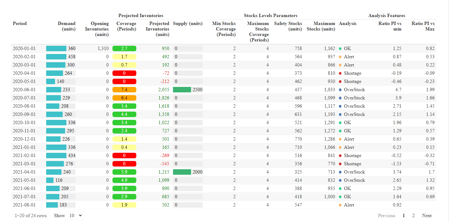
a) Table
Now we’re going to apply the proj_inv() function.
Same with the function light_proj_inv(), it will allow to calculate 2 features for the DFU :
projected inventories
projected coverages, based on the Demand Forecasts
And also 5 new features :
Safety.Stocks : the projected Safety Stocks quantity, in units
Maximum.Stocks :the projected Maximum Stocks quantity, in units
PI.Index : a indicator, to inform whether the Projected Inventories are in OverStock (above the Maximum Stock target), in Alert (below the Safety Stock target), in Shortage (no stocks), or OK (between the 2 targets)
Ratio.PI.vs.min : a comparison of the Projected Inventories vs Safety Stocks target
Ratio.PI.vs.Max : a comparison of the Projected Inventories vs Safety Stocks target
We also can notice that the minimum and maximum stocks coverages, initially expressed in Periods (of coverage) are converted in units.
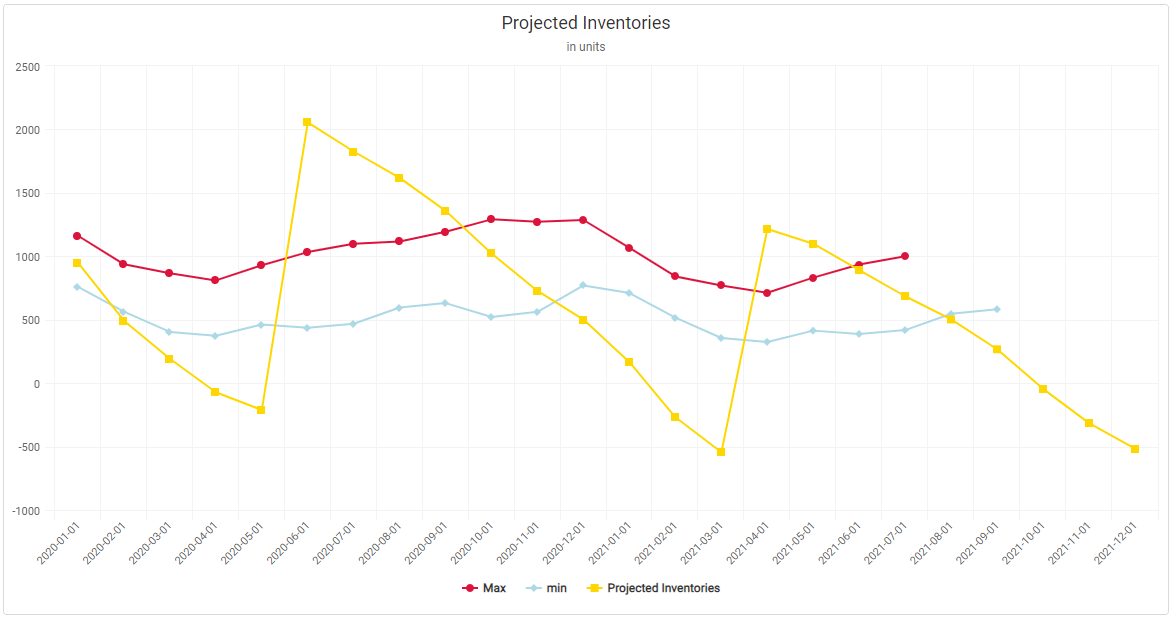
It will quite useful to chart the projected inventories vs those 2 thresholds, to display where our [Projected.Inventories] stand vs those targets.
The [PI.Index] and the 2 ratios [Ratio.PI.vs.min] & [Ratio.PI.vs.Max] are useful to filter the data on the relevant products with issues, displaying quickly which products have issues, when and how much (vs targets).
b) Chart
On top of seeing when we have stocks, and when we project to be in shortage, the idea is to quickly visualize the evolution of our projected inventories, and compare them vs min & max targets levels.
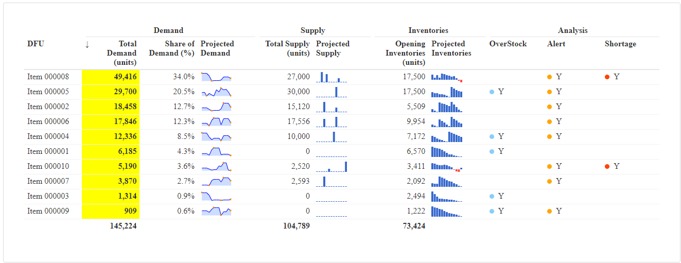
c) Cockpit
If we perform a calculation for several products, we can use a cockpit to get an overview.
The 3 columns of the right inform us whether one item has a risk of shortage, alert (below minimum stock target) or overstock (above maximum stock target) over a selected horizon.
3) Table w/ Constrained Demand
Let’s calculate the Constrained Demand, using the function const_dmd() .
This function actually calculates 2 things :
the projected inventories and coverages, just like the function light_proj_inv()
and also, based on those projections : the actual (possible) Demand
- which is then the constrained Demand
When we look at the projected inventories, we can see that we will be late (negative projected inventories) to supply some Demand.
The idea through this function is then to know the constrained Demand : how much Demand can be supplied (answered) and when, based on the projected inventories.
The table below displays :
in blue the initial (unconstrained) Demand
in yellow the possible (constrained) Demand
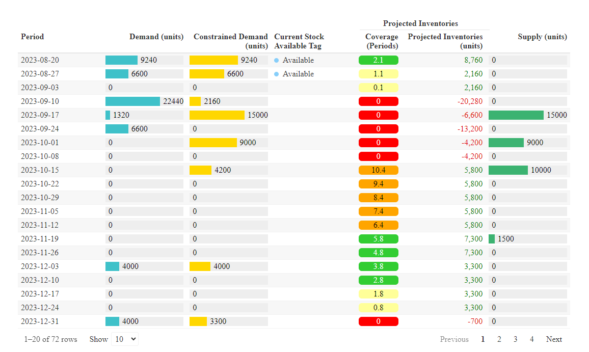
We can see that the [Constrained Demand] is different from the original, unconstrained Demand :) (obviously!)
There is also another useful insight : [Current Stock Available Tag]
it informs the quantity of the original unconstrained Demand which can be supplied, considering the current stocks available (i.e the Opening)
the Opening Inventories are here of 18.000 units, which are enough stocks to supply the Demand of the 2 first weeks
4) Calculated Replenishment Plan
Now let’s apply the drp() function to a demo dataset.
As a result, we obtain 5 new variables :
Safety.Stocks : the projected safety stocks, in units
Maximum.Stocks : the projected maximum stocks, in units.
- Maximum Stock = Safety Stocks (SSCov) + Frequency of Supply (DRPCovDur)
DRP.Calculated.Coverage.in.Periods : the calculated projected inventories, expressed in periods of coverage
DRP.Projected.Inventories.Qty : the calculated projected inventories, based on the [DRP.plan]
DRP.plan : the calculated Replenishment Plan
in the Frozen Horizon : the existing plan, which is “frozen”
in the Free Horizon : the calculated plan, based on the parameters (SSCov, DRPCovDur, MOQ)
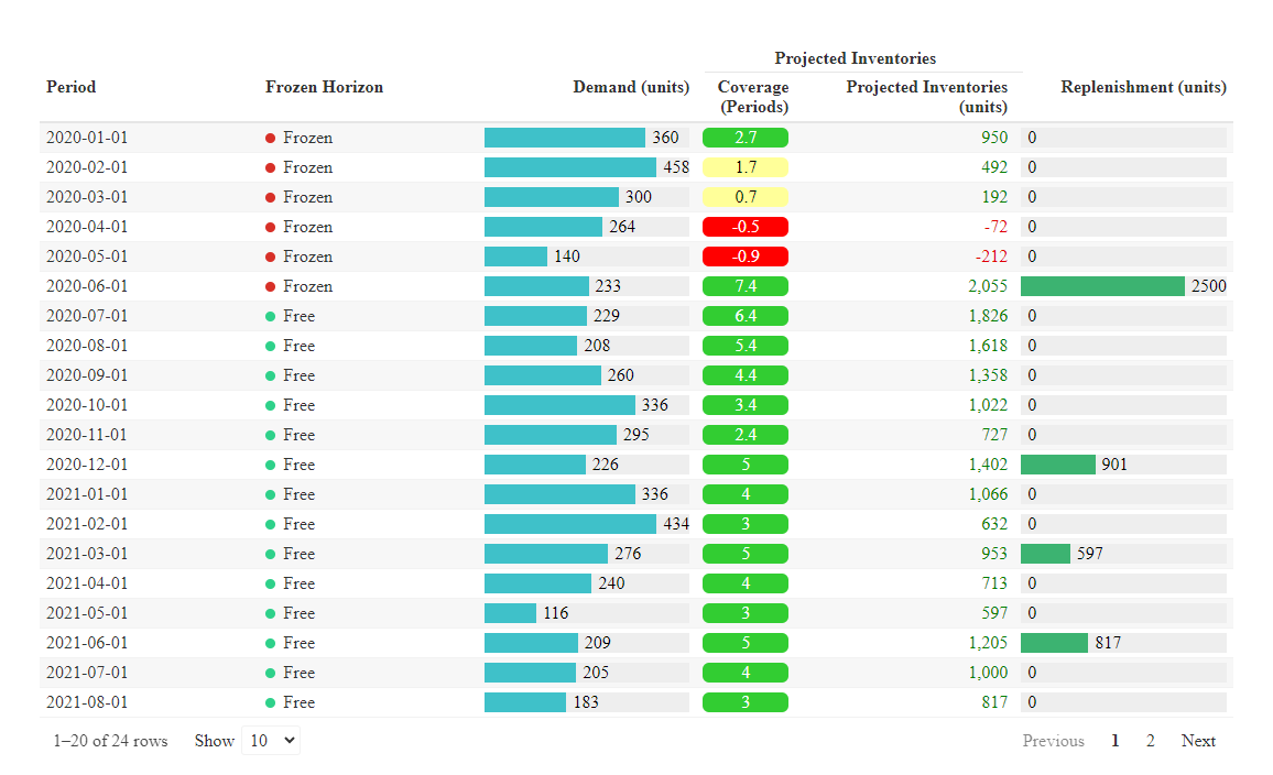
a) Table
The table below displays :
the Frozen Horizon
the calculated Replenishment Plan
and the related projected inventories & coverages
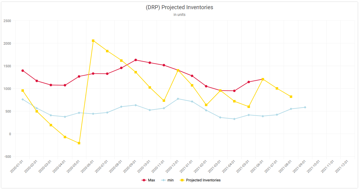
b) Chart
The chart below displays the calculated projected inventories vs 2 references :
minimum stocks : when we reach it we get a new replenishment
maximum stocks : equals to minimum stocks + Replenishment Frequency
The calculated projected inventories fluctuate between those 2 levels.
5) Conversion Monthly to Weekly buckets
We’re going to use here the month_to_week() function.
This function allows to split a Demand (for ex.: Sales Forecasts) from monthly into weekly buckets.
We need a dataset with the 3 variables to use this function :
a Product: it’s an item, a SKU (Storage Keeping Unit), or a SKU at a location, also called a DFU (Demand Forecast Unit)
a Period of time : here in monthly buckets
a Demand : could be some sales forecasts, expressed in units
In the picture below we have splitted the initial monthly demand (left chart) into weekly buckets (right chart).
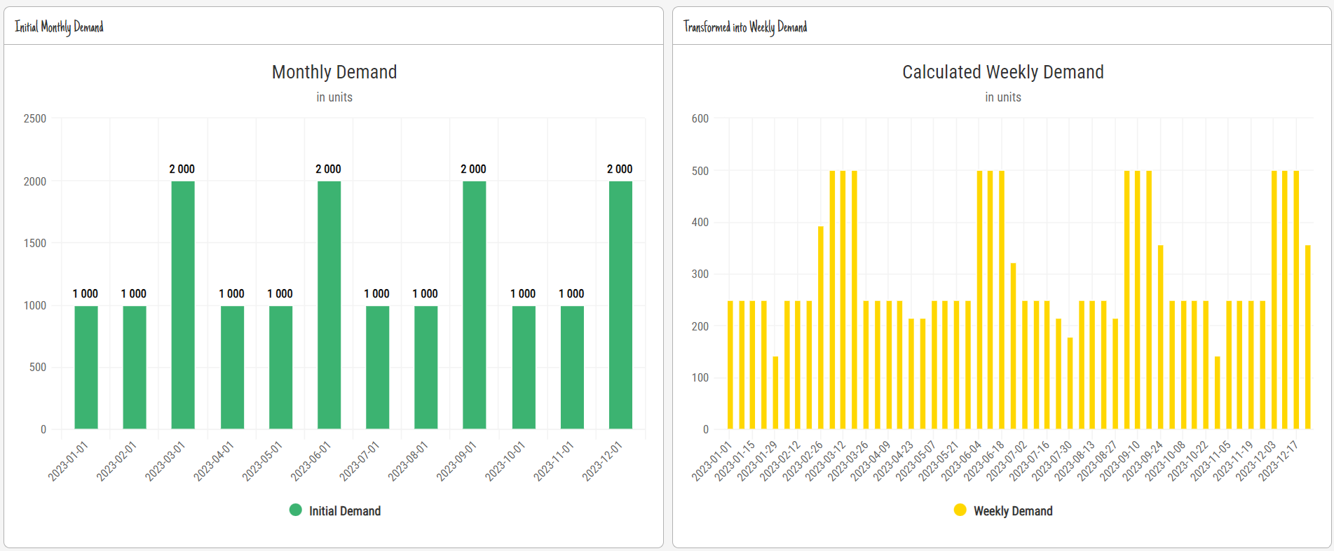
Note : by default, the split is performed evenly for each week.